From satellite pixels to sampling decisions
Vision transformers and active learning for rodent-borne zoonoses
5 November 2026
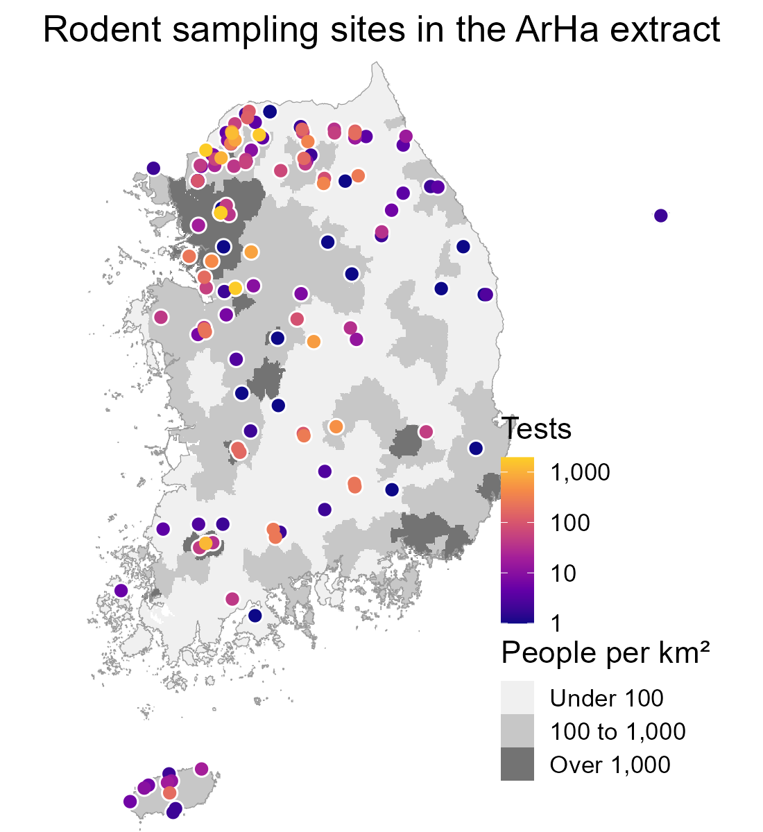
Surveillance is reactive, so our data are biased
- Rodents are mostly sampled after outbreaks, or where trapping is convenient
- Models trained on these data learn where people looked, not only where the hazard is
- The project treats surveillance as a question of where new data would reduce uncertainty most
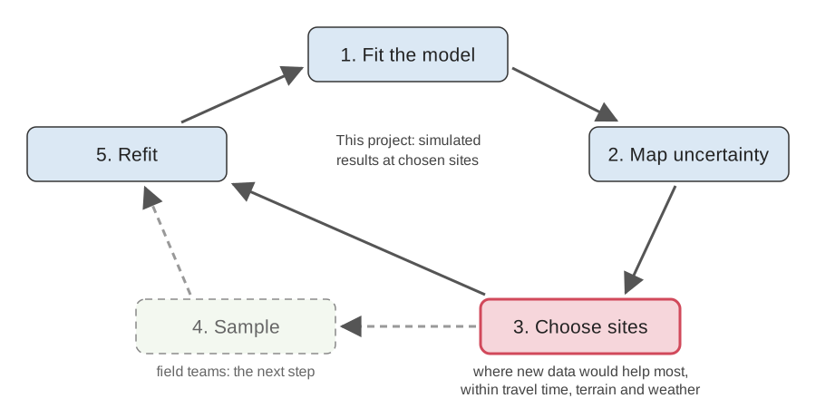
The pipeline on one slide
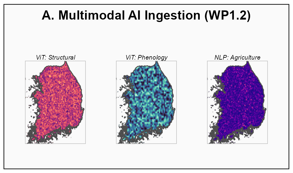
1. Landscape features from satellites
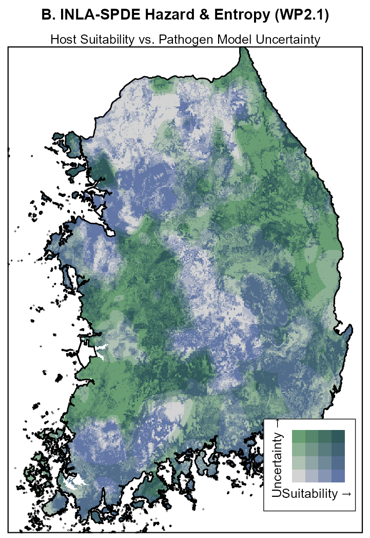
2. Hazard and how sure we are
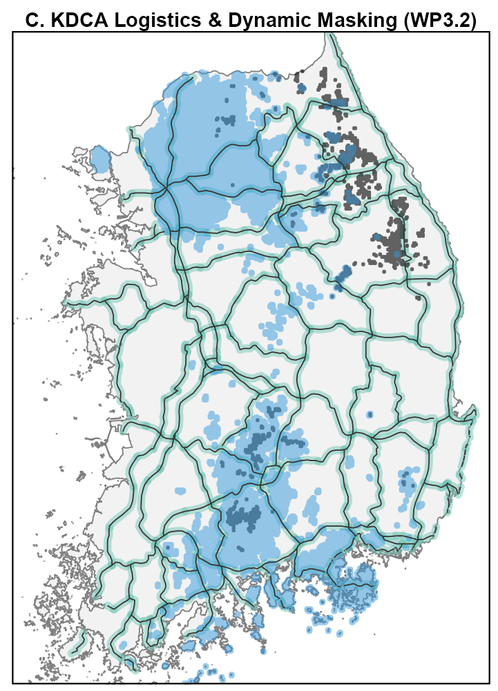
3. Where teams can reach
4. Where to sample next
Before transformers: bands and indices
- Glass et al. 2000: three Landsat bands plus elevation, from the year before the 1993 outbreak, retrospectively identified hantavirus pulmonary syndrome case sites
- A model using only the vegetation index (NDVI) fitted poorly in that sparse, semi-arid landscape
- Rich spectral information carries more than any single index
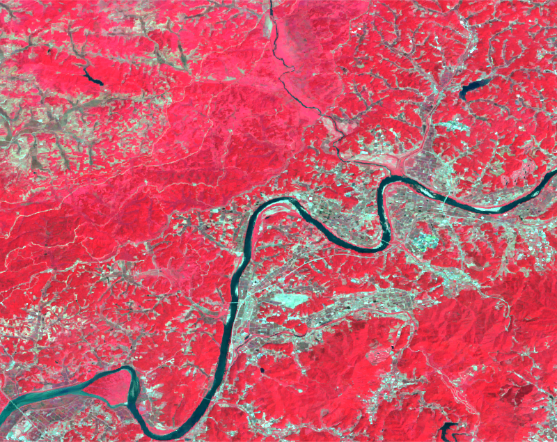
What a vision transformer is
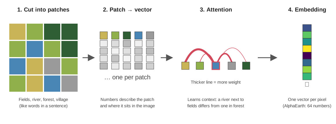
- The image is cut into small patches, like words in a sentence
- Each patch becomes a vector of many numbers from all its bands, so two forests no longer share one label
- Attention updates each patch using every other patch, so the same river differs next to fields or in forest
- The output is one vector per pixel: a learned summary of the place and its surroundings
What an embedding is
- AlphaEarth Foundations: 64 numbers for every 10 m pixel, one layer per year, 2017 to 2025
- The numbers summarise what the landscape looks like across sensors and seasons
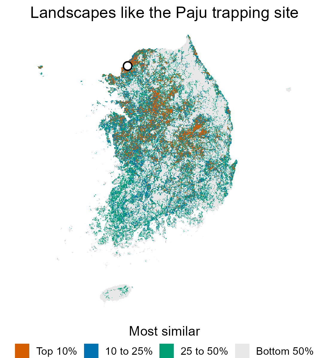
- Similar landscapes have similar embeddings, whatever their land-cover label
What the similar places are made of
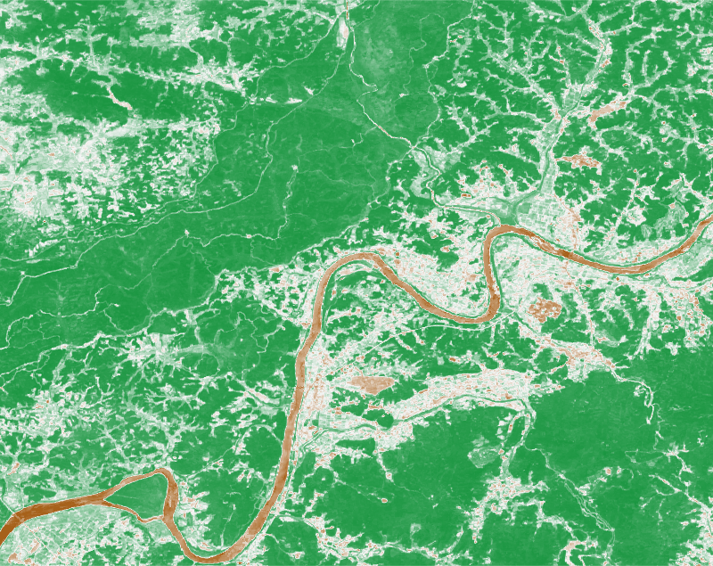
- The more similar to Paju, the more cropland and the less forest
- Half the top 10% are crop and forest mosaics like Paju, against 5% of the bottom half
- Yet the top 10% is still half tree cover on average: similar is not just “more fields”
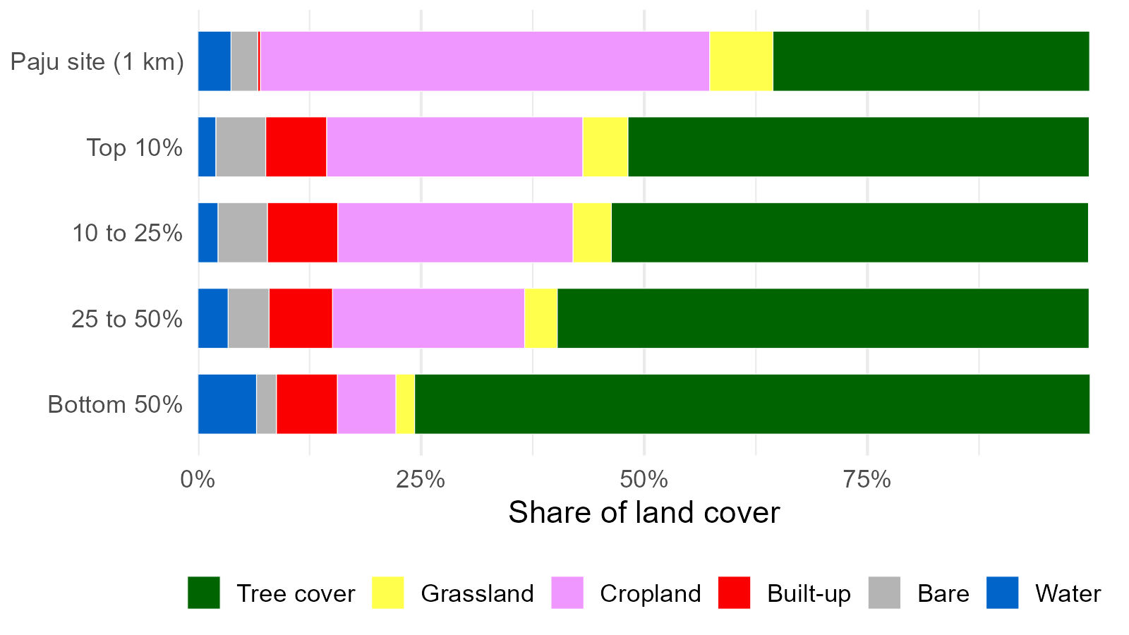
Average land cover of the cells in each similarity band. ESA WorldCover 2020
Three ways to describe the same cell
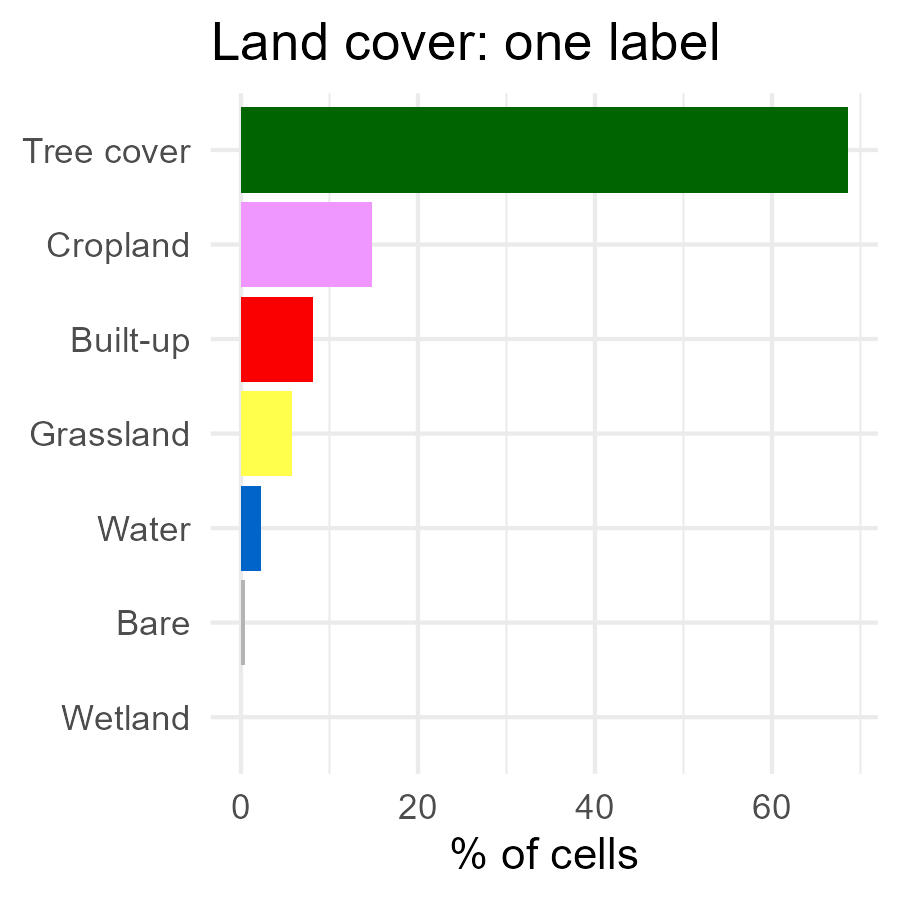
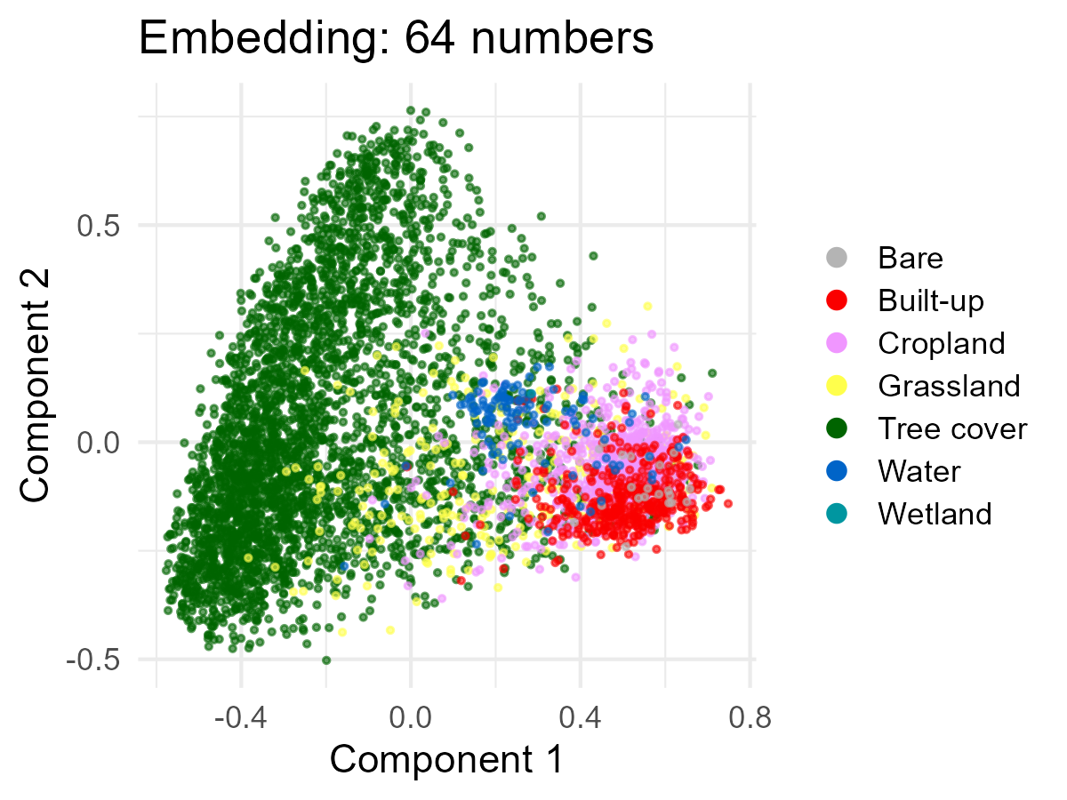
- A label puts two-thirds of the country in one box (tree cover)
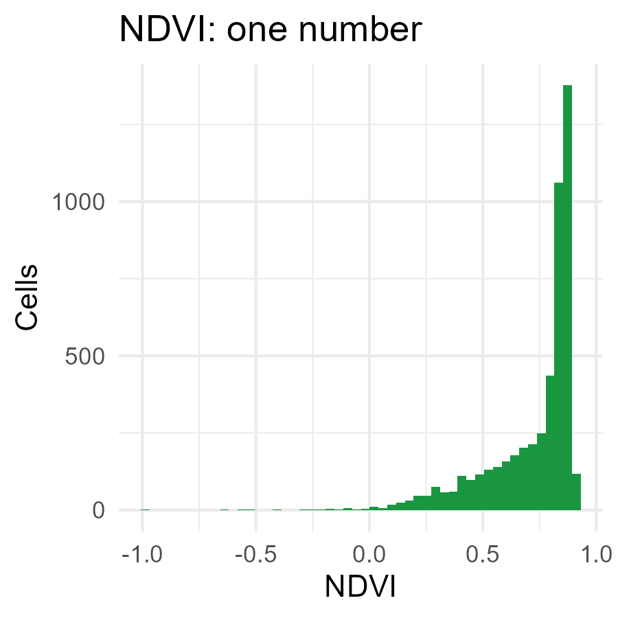
- NDVI puts over half the cells between 0.8 and 0.9, where it saturates
- The embedding keeps differences within a class, so a model can learn which of them matter for rodents
- Whether that predicts better is something we test, not assume (comparison with standard covariates)
Where should the next trap go?
We trap to learn where human cases will occur. Which sites teach us most?
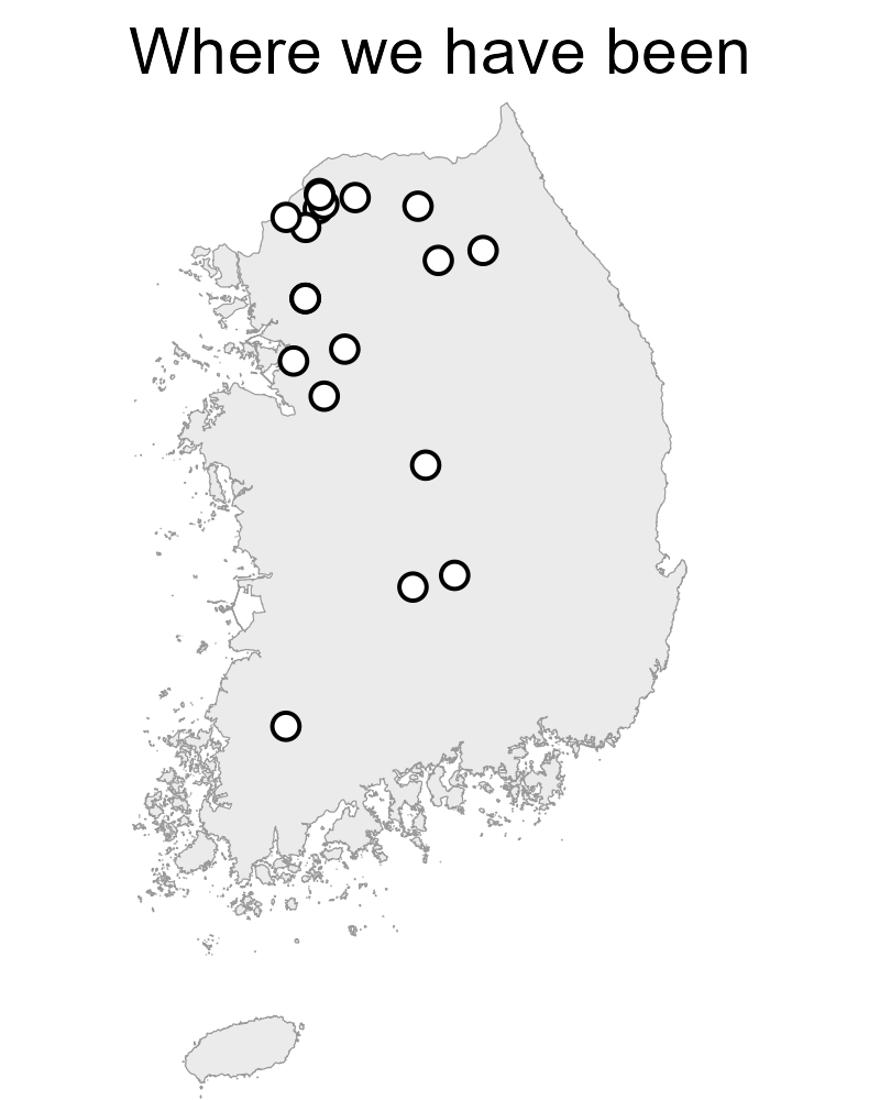
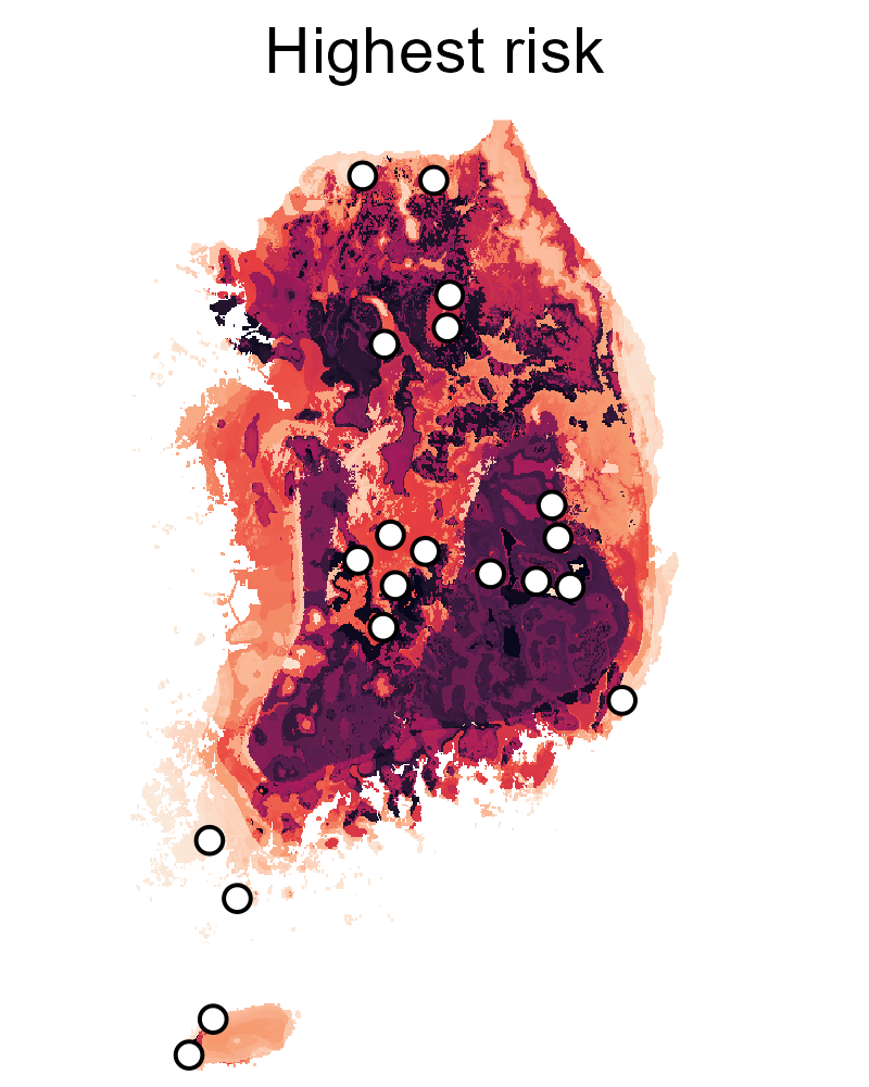
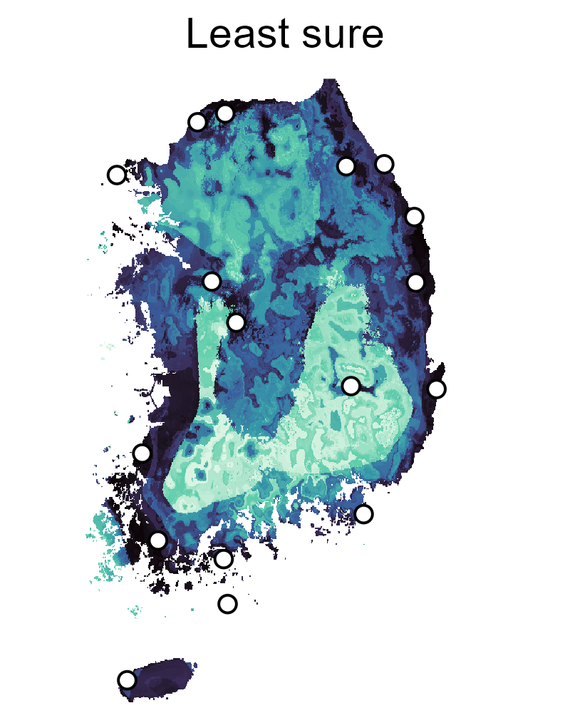
Return to past sites: change over time, or breadth?
Highest predicted risk: does the model hold up?
Where we can’t tell high from low: can the model improve?
Not all uncertainty is worth a trap
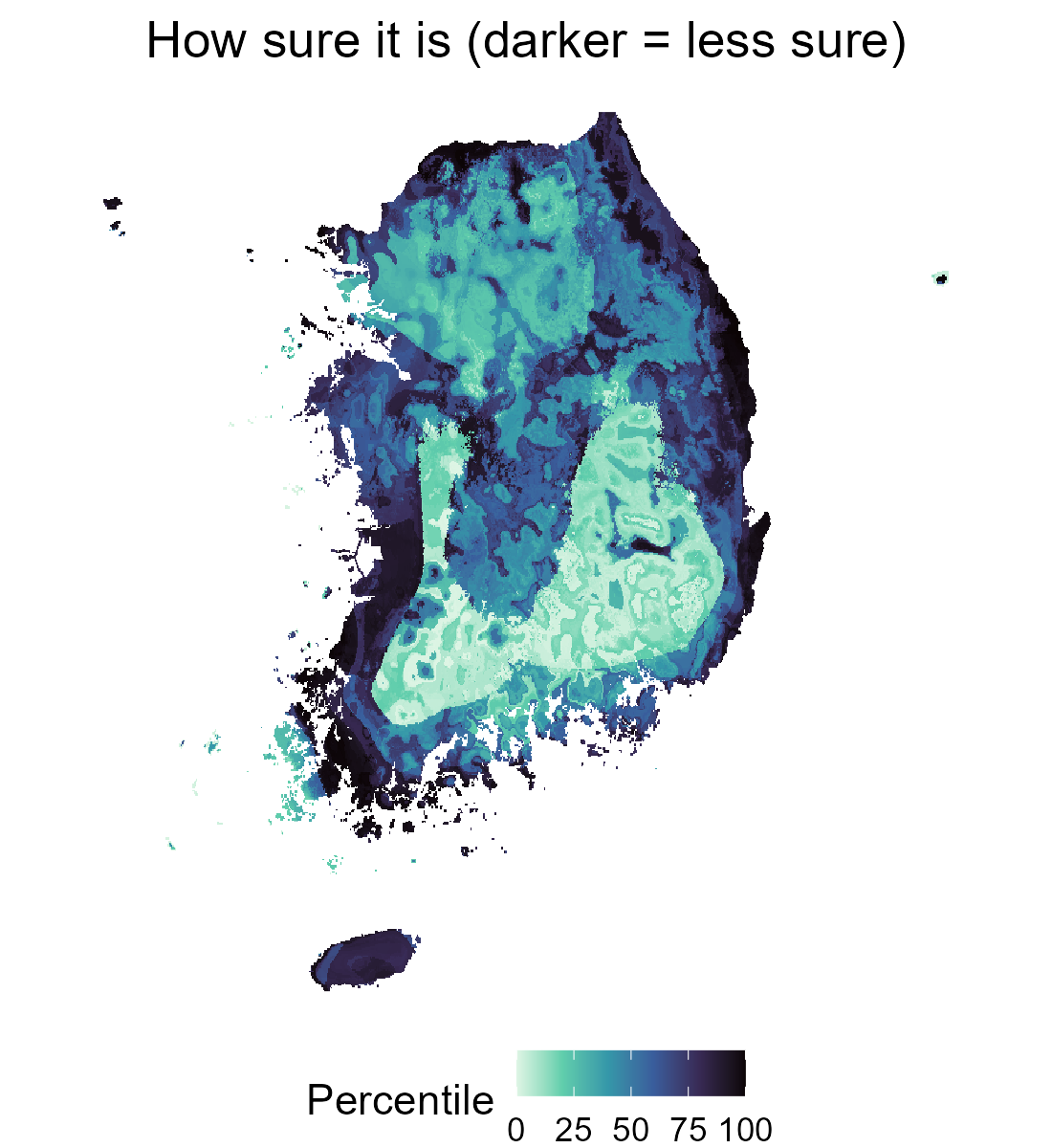
- Reducible: we haven’t looked there, or anywhere like it. More samples shrink it
- Irreducible: cells that look alike to the model still differ. Trapping one tells you about that cell, not the next one like it
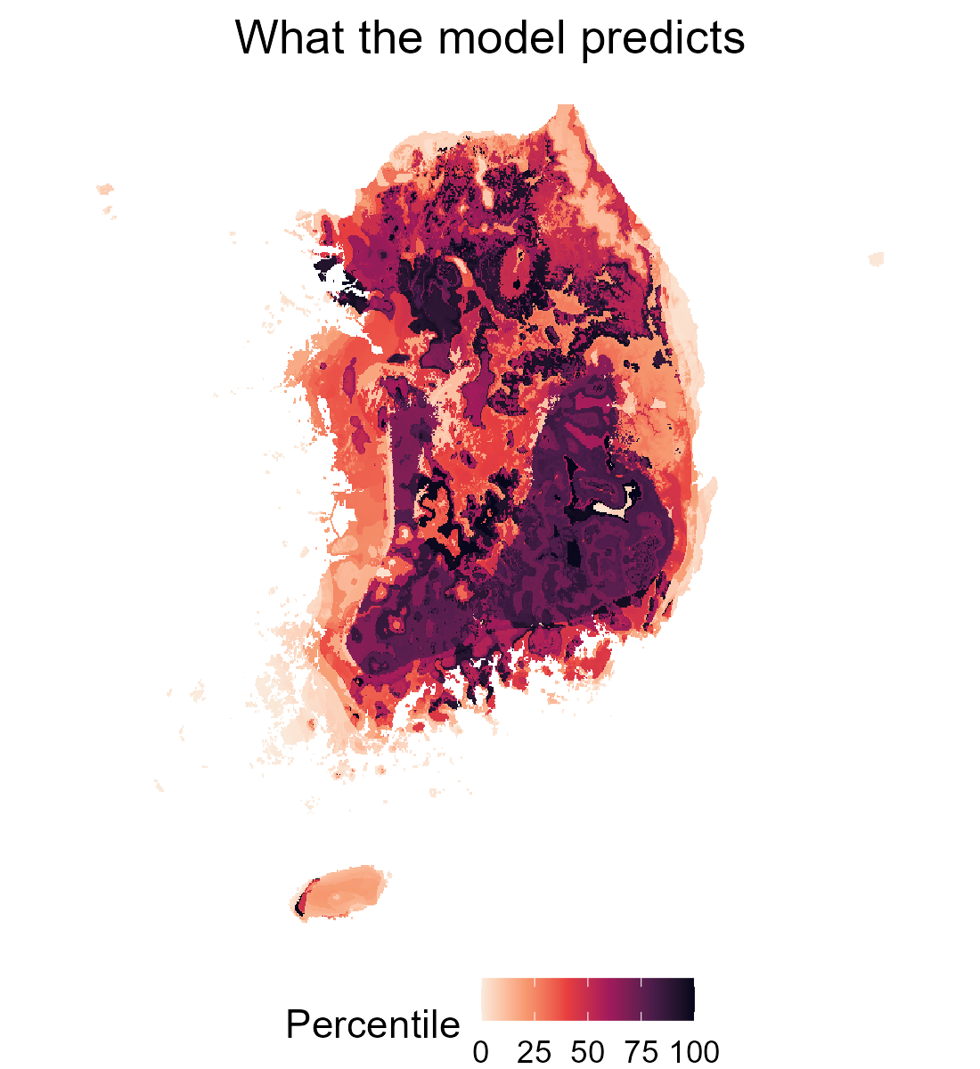
- This map is mostly the second kind: highest where suitability is middling, near zero where the model is confident, even with no data nearby
- Downscaling to 1 km gives both kinds for human incidence (Python et al. 2022); site choice should use the reducible part
The active learning loop
Example 1: hotspots with fewer samples
- Andrade-Pacheco et al. 2020: schistosomiasis and lymphatic filariasis in four countries
- Sites chosen by the entropy of the probability of being a hotspot, spread out within each batch
- Matched the accuracy of 100 random sites with 7 to 50% of the samples
- Trade-off: better at classifying hotspots, worse at overall prediction error
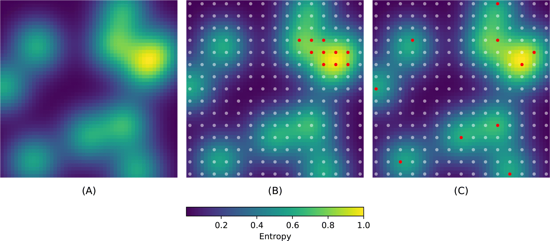
Left: uncertainty. Middle: the most uncertain sites, which cluster. Right: the batch spread out. Figure 3 from Andrade-Pacheco et al. 2020, Sci Rep, CC BY 4.0
Example 2: South Korea, same hosts and data
- Catchen et al. 2026: host distribution models plus prevalence data from ArHa
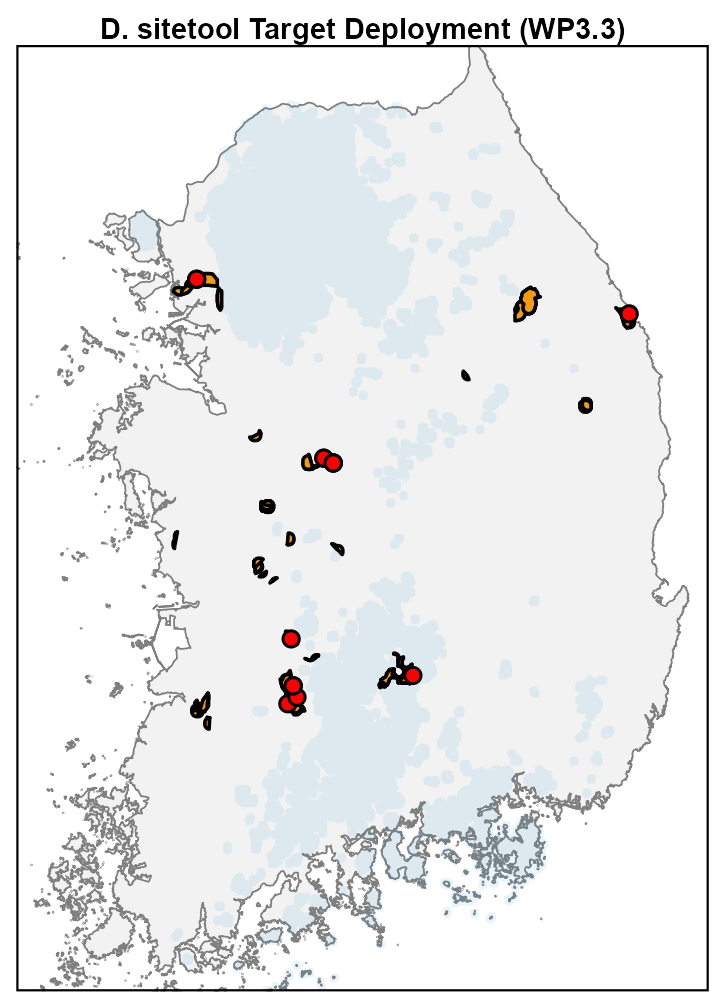
- Discovery sampling where host presence is uncertain (north-west, around Seoul)
- Prevalence sampling where hosts are certain but prevalence is not (south-east)
- Our code base starts from this case study
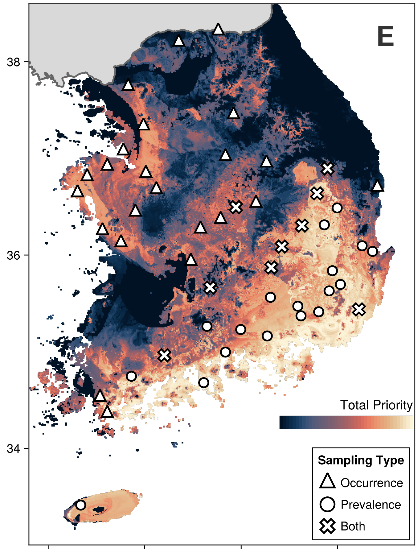
Panel E of the South Korea figure, Catchen et al. 2026, PLOS Ecosystems, CC BY 4.0
Example 3: tested in the field
- Bengsen et al. 2026: wild pigs across New South Wales, 1,964 animals over two years
- Search value updated every three months from the sampling actually done: a sampled cell drops, even if its risk stays high
- Sites balance search value against spread; 74 to 88% of sampled cells were still high risk
- Built for foot-and-mouth disease, but also found Japanese encephalitis virus at sites other JEV models rated low to moderate risk
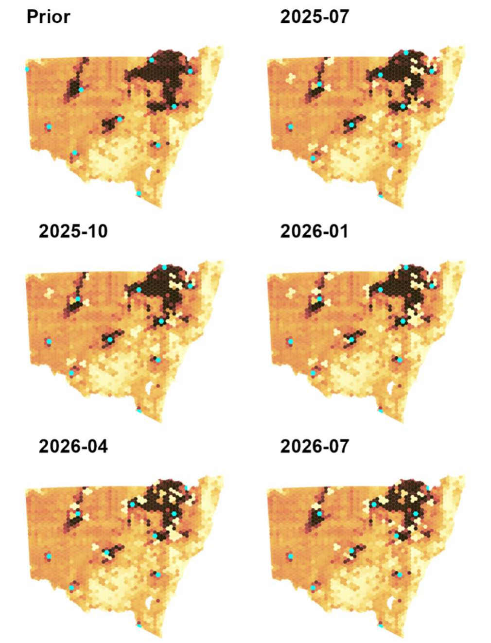
Search value, updated every three months; cyan = chosen cells. Figure 3 from Bengsen et al. 2026, bioRxiv, CC BY-NC-ND 4.0
Where this leaves us
- Surveillance data record where people looked, so a model trained on them learns the looking as well as the hazard
- Embeddings describe a landscape without us choosing the variables first, and we test whether that predicts better
- Uncertainty is a map in its own right, and the part sampling can shrink is the part worth a trap
- The loop is only useful if it survives the field, so logistics and simulation come before any sampling plan